6. Demand curves#

TIMES-NZ models electricity demand in “timeslices” each year. These split the year into 4 seasons, 2 day types (weekends and weekdays), and three times of day (day, night, and peak), for a total of 24 different times of year. We define peak as the hour from 6-7pm. This is important for modelling the interaction between intermittent electricity supply and variable electricity demand.

6.1. Residential load curve data#

To model the effective shape of residential demand according to these parameters, we use data from the 2021 Residential Baseline Study[1], which models different patterns of electricity demand behaviour for residential users across Australia and New Zealand. This data does not distinguish space heating from space cooling, instead categorising this demand all under one category of “Space Conditioning”. To apply this to TIMES-NZ, we disaggregate “Space Conditioning” into heating and cooling demand according to the assumptions in Table 53. These assumptions are not based on detailed modelling or analysis but are intended to be sufficiently representative.

Table 53 Assumed heating shares of Space Conditioning demand#
Season	Heating %	Cooling %
Spring	90%	10%
Summer	0%	100%
Autumn	90%	10%
Winter	100%	0%

RBS end use categories are then assigned to TIMES-NZ categories as outlined in Table 54.

Table 54 Residential Baseline Study and TIMES-NZ use categories#
TIMES-NZ Category	RBS Category
Refrigeration	White goods
Space Cooling	Space conditioning (cooling share)
Low Temperature Heat (<100 C), Clothes Drying	White goods
Low Temperature Heat (<100 C), Clothes Washing	White goods
Low Temperature Heat (< 100 C), Dishwashers	White goods
Low Temperature Heat (<100 C), Space Heating	Space conditioning (heating share)
Low Temperature Heat (<100 C), Water Heating	Water heating
Intermediate Heat (100-300 C), Cooking	Cooking
Electronics and other Electrical Uses	IT&HE
Lighting	Lighting

6.2. Ripple control adjustments and scenario differentiation#

We modify the peak demand of hot water heating to allow for ripple controlled hot water. We assume that 50% of electric hot water cylinders are currently operating with ripple control[2]. The relevant demand is shifted to night in the model.

For the Shift scenario, we assume that further investment in smart meters, time of use pricing, and other smart solutions increase this rate to 90% by 2050, further reducing peak load.

6.3. Resulting peak demand#

The resulting average demand curves for weekday loads are demonstrated in Fig. 4.

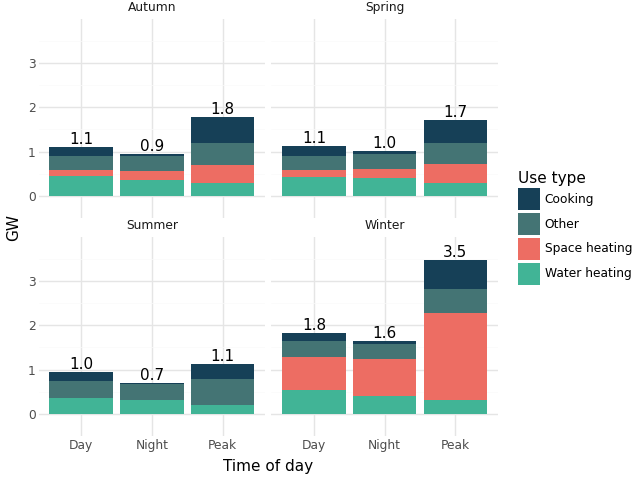
Fig. 4 Residential weekday load curves 2023#

6.4. Residential space heating peaks#

Because our winter peak period still covers 66 hours (1 hour out of every weekday in winter), the average load during this period is around lower than actual peak for any given year. We assume the actual residential peak demand is closer to 4GW, allowing for the possibility of increased space heating demand due to cold snaps. We therefore include a residential space heating factor by assumption: increasing the demand for space heating by 25% when calculating the model’s peak constraint. Note that this demand-side factor of the peaking constraint is additional to other components of the model constraint, such as the peak capacity contributions[3].